Introduction
Vision Transformers (ViT) have emerged as a groundbreaking architecture in the field of computer vision, challenging the long-standing dominance of Convolutional Neural Networks (CNNs).
Introduced by Alexey Dosovitskiy and his team at Google Research in 2020, ViTs apply the transformer architecture, originally designed for natural language processing tasks, to image recognition problems.
Traditional CNNs have been the cornerstone of image processing for years, but they have limitations in capturing global context and long-range dependencies. ViTs address these limitations by leveraging the self-attention mechanism, which allows the model to consider the entire image at once, rather than just local regions.
Background: From CNNs to Transformers
To appreciate the significance of Vision Transformers, it’s crucial to understand the context in which they emerged. For nearly a decade, Convolutional Neural Networks (CNNs) have been the go-to architecture for image-related tasks. CNNs excel at capturing local spatial relationships in images through their use of convolutional filters. However, they struggle with modeling long-range dependencies efficiently.
CNNs work by applying a series of convolutional filters to an image, each filter looking for specific features like edges, textures, or more complex patterns. This approach is inherently local – each layer in a CNN only looks at a small portion of the input at a time. While this is effective for many tasks, it can miss important global context.
Transformers, on the other hand, were initially designed for sequence-to-sequence tasks in natural language processing. Their key innovation is the self-attention mechanism, which allows the model to weight the importance of different parts of the input when processing each element. This mechanism enables transformers to capture long-range dependencies effectively.
In the context of language, this means a transformer can easily relate words at the beginning of a sentence to words at the end, something that’s more challenging for traditional recurrent neural networks. When applied to images, this translates to the ability to relate distant parts of an image, capturing global context more effectively than CNNs.
The success of transformers in NLP tasks prompted researchers to explore their potential in other domains, including computer vision. This exploration led to the development of Vision Transformers, which adapt the transformer architecture to work with image data.
Architecture of Vision Transformers
Vision Transformers adapt the transformer architecture to work with image data. The key steps in this process are:
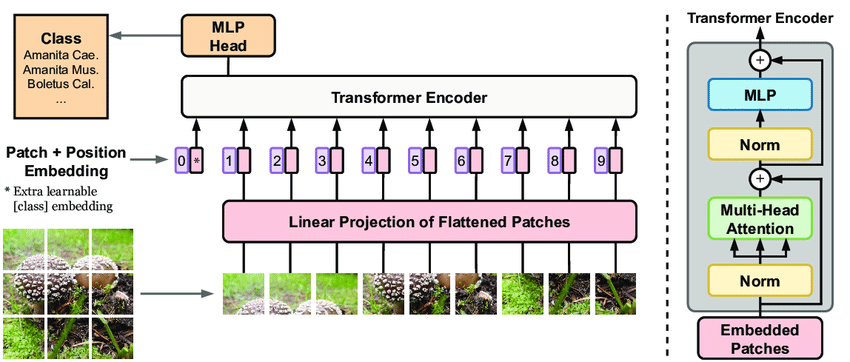
- Image Patching: The input image is divided into fixed-size patches.
- Linear Embedding: Each patch is flattened and linearly embedded.
- Position Embedding: Positional information is added to the patch embeddings.
- Transformer Encoder: The embedded patches are processed by a standard transformer encoder.
- Classification Head: The output of the encoder is used for classification.
Image Patching
The first step in processing an image with a Vision Transformer is to divide it into fixed-size patches. Given an image $x \in \mathbb{R}^{H \times W \times C}$, where $H$, $W$, and $C$ are the height, width, and number of channels respectively, we split it into $N$ patches where $N = HW/P^2$. Each patch $x_p \in \mathbb{R}^{P \times P \times C}$ has a resolution of $P \times P$. This patching operation can be seen as a form of tokenization, similar to how words are tokenized in NLP tasks. Each patch becomes a “visual word” that the transformer will process.
The choice of patch size is an important hyperparameter. Smaller patches allow for finer-grained analysis but increase computational complexity, while larger patches reduce complexity but may lose fine details. Typical patch sizes range from 14x14 to 32x32 pixels.
For example, if we have a 224x224 pixel RGB image and choose a patch size of 16x16, we would end up with 196 patches (14x14 grid of patches), each represented as a 768-dimensional vector (16 * 16 * 3 = 768).
Linear Embedding
After patching, each patch is flattened and linearly projected to a D-dimensional embedding space. This is done using a learnable linear projection $E \in \mathbb{R}^{(P^2 \cdot C) \times D}$ The resulting patch embeddings are denoted as:
$$z_0 = [x_p^1E; x_p^2E; … ; x_p^NE]$$
where $x_p^i$ is the i-th flattened patch and $z_0 \in \mathbb{R}^{N \times D}$ is the sequence of patch embeddings.
This linear embedding serves multiple purposes:
- It allows the model to learn a meaningful representation of the image patches in a high-dimensional space.
- It maps the variable-sized patches (depending on the image size) to a fixed-dimensional space that the transformer can process.
- It can be seen as learning a set of filters, similar to the first layer of a CNN, but applied globally to each patch.
The dimension D is typically chosen to match the internal dimension of the transformer model, often 768 or 1024 in practice.
Position Embedding
Unlike CNNs, which inherently capture spatial information through their convolutional operations, transformers don’t have a built-in sense of spatial relationships. To compensate for this, position embeddings are added to the patch embeddings.
A learnable position embedding $E_{pos} \in \mathbb{R}^{(N+1) \times D}$ is added to the patch embeddings. The "+1" in the dimension accounts for a special “classification token” that’s prepended to the sequence of patch embeddings.
This results in:
$$z_0 = [x_{class}; x_p^1E; x_p^2E; …; x_p^NE] + E_{pos}$$
where $x_{class}$ is the learnable classification token.
The position embeddings play a crucial role:
- They provide the model with information about the spatial arrangement of the patches.
- Unlike in NLP transformers where positions are usually encoded using fixed sinusoidal functions, ViTs typically use learnable position embeddings, allowing the model to adapt to the 2D structure of images.
- The addition of position embeddings to the patch embeddings allows the model to distinguish between identical patches at different locations in the image.
The classification token ($x_{class}$) is a special learned vector that’s prepended to the sequence of patch embeddings. Its final representation after passing through the transformer encoder is used for classification tasks, serving a similar purpose to the [CLS] token in BERT for NLP tasks.
Transformer Encoder
The core of the Vision Transformer is the transformer encoder. It consists of alternating layers of multihead self-attention (MSA) and multilayer perceptrons (MLP). Layer normalization (LN) is applied before each block, and residual connections are employed around each block.
The computation in the L-layer transformer encoder proceeds as follows:
$$\begin{aligned} z_0’ &= [x_{class}; x_p^1E; x_p^2E; …; x_p^NE] + E_{pos} \end{aligned}$$
$$\begin{aligned} z_l’ &= MSA(LN(z_{l-1})) + z_{l-1}, &l = 1…L \end{aligned}$$
$$\begin{aligned} z_l &= MLP(LN(z_l’)) + z_l’, &l = 1…L \end{aligned}$$
The multihead self-attention operation is the key component that allows the model to capture relationships between different parts of the image. For each attention head, the input is projected into query (Q), key (K), and value (V) vectors. The attention weights are computed as:
$$Attention(Q, K, V) = softmax(\frac{QK^T}{\sqrt{d_k}})V$$
where $d_k$ is the dimension of the key vectors. The $\frac{1}{\sqrt{d_k}}$ scaling factor is used to counteract the effect of the dot product growing large in magnitude for high dimensions.
Let’s break down the transformer encoder further:
-
Multihead Self-Attention (MSA): This allows the model to attend to different parts of the input simultaneously. Each head can focus on different relationships between patches.
-
Layer Normalization (LN): This helps stabilize the learning process by normalizing the inputs to each layer.
-
Multilayer Perceptron (MLP): This is typically a simple feed-forward network applied to each position separately and identically. It allows for non-linear transformations of the features.
-
Residual Connections: These help in training deep networks by allowing gradients to flow more easily through the network.
The self-attention mechanism is particularly powerful because it allows each patch to interact with every other patch, capturing global relationships in the image. This is in contrast to CNNs, where each layer only looks at a local neighborhood of pixels.
Classification Head
After the transformer encoder processes the sequence of patch embeddings, the final classification is performed using the representation of the classification token. A simple linear layer is typically used as the classification head:
$$y = MLP(z_L^0)$$
where $z_L^0$ is the final hidden state corresponding to the classification token.
The classification head is straightforward compared to the rest of the architecture. It takes the final representation of the classification token, which has aggregated information from the entire image through the self-attention process, and maps it to the output classes.
This simplicity is part of the elegance of the ViT architecture – all the heavy lifting is done by the transformer encoder, and the classification is a simple linear projection of the resulting representation.
Training and Fine-tuning
Vision Transformers are typically pre-trained on large datasets and then fine-tuned on specific tasks. The pre-training is often done using a supervised approach on large-scale datasets like ImageNet-21k or JFT-300M. During pre-training, the model learns to extract meaningful features from images that can be useful for a wide range of tasks.
The pre-training process is crucial for ViTs, perhaps even more so than for CNNs. This is because ViTs lack the inductive biases that CNNs have (such as translation invariance), so they need to learn these properties from data. Pre-training on a large, diverse dataset allows the ViT to learn general visual features that can be applied to many different tasks.
The fine-tuning process for ViTs is similar to that of other pre-trained models:
- The pre-trained ViT is loaded, usually without the final classification layer.
- A new classification layer is added, with the number of outputs matching the number of classes in the target task.
- The model is then trained on the target dataset. Often, a lower learning rate is used for the pre-trained weights, with a higher learning rate for the new classification layer.
One of the strengths of ViTs is their ability to transfer well to a wide range of tasks with minimal fine-tuning. This is likely due to the global nature of the features they learn during pre-training.
Advantages of Vision Transformers
Vision Transformers offer several advantages over traditional CNN architectures:
-
Global Context: The self-attention mechanism allows ViTs to capture long-range dependencies and global context more effectively than CNNs. This means ViTs can more easily relate distant parts of an image, which can be crucial for tasks that require understanding the overall scene or object relationships.
-
Scalability: ViTs have shown impressive scaling properties, with performance continuing to improve as model size and training data increase. This is similar to what has been observed with language models, where larger models trained on more data consistently perform better.
-
Transfer Learning: Pre-trained ViTs have demonstrated strong transfer learning capabilities, performing well on a wide range of tasks with minimal fine-tuning. This makes them versatile and potentially more cost-effective for organizations dealing with multiple vision tasks.
-
Interpretability: The attention maps produced by ViTs can provide insights into which parts of the image the model is focusing on for its decisions. This can be valuable for understanding and debugging model behavior.
-
Unified Architecture: ViTs provide a unified architecture that can be applied to various vision tasks beyond just classification, including object detection and segmentation. This simplifies the model design process across different tasks.
-
Efficiency at Scale: While ViTs can be computationally expensive to train, they can be more efficient than CNNs for very large models. This is because self-attention operations can be optimized more effectively on modern hardware than convolutions for large model sizes.
Challenges and Limitations
Despite their advantages, Vision Transformers also face some challenges:
-
Data Hunger: ViTs typically require larger datasets for training compared to CNNs, especially when training from scratch. This is because they need to learn basic visual features that are built into the architecture of CNNs. For smaller datasets, CNNs often still outperform ViTs unless specific techniques are used to address this limitation.
-
Computational Cost: The self-attention mechanism in ViTs has a quadratic complexity with respect to the number of patches, which can be computationally expensive for high-resolution images. This means that processing very large images or scaling to very high resolutions can be challenging.
-
Lack of Inductive Biases: Unlike CNNs, which have built-in inductive biases for processing visual data (like translation invariance), ViTs need to learn these properties from data, which can require more training. This is why pre-training on large datasets is so important for ViTs.
-
Positional Information: While position embeddings help, capturing and utilizing spatial relationships as effectively as CNNs remains a challenge for ViTs. The discrete nature of the patch-based approach can sometimes lead to artifacts or reduced performance on tasks that require fine-grained spatial understanding.
-
Model Size: Competitive ViT models are often larger than their CNN counterparts, which can make them challenging to deploy in resource-constrained environments like mobile devices.
-
Training Instability: ViTs can sometimes be more challenging to train than CNNs, requiring careful tuning of hyperparameters and learning rates. The lack of inductive biases can lead to more pronounced overfitting on smaller datasets.
Researchers are actively working on addressing these limitations, leading to numerous variations and improvements on the original ViT architecture.
Recent Developments and Variations
Since the introduction of the original ViT, numerous variations and improvements have been proposed:
-
DeiT (Data-efficient Image Transformers): This variant introduces a teacher-student strategy to train ViTs more efficiently on smaller datasets. DeiT uses a CNN as a teacher to provide additional supervision during training, allowing the ViT to learn more effectively from limited data. This addresses one of the main limitations of the original ViT – its data hunger.
-
Swin Transformer: This hierarchical approach uses shifted windows to compute self-attention, allowing for better efficiency and applicability to dense prediction tasks. The Swin Transformer computes self-attention within local windows, and these windows are shifted between successive layers. This approach reduces computational complexity and makes it easier to apply ViTs to tasks like object detection and segmentation.
-
MLP-Mixer: This architecture replaces the self-attention layers with simple MLPs, demonstrating that the patch-based approach, rather than self-attention, might be the key innovation of ViTs. MLP-Mixer alternates between MLPs applied across channels and MLPs applied across spatial locations. This simplification can lead to faster training and inference while maintaining competitive performance.
-
CoAtNet: This hybrid approach combines convolutions and self-attention, aiming to get the best of both worlds. It uses convolutions in the earlier layers to efficiently process low-level features, and self-attention in the later layers to capture global context. This combines the efficiency and inductive biases of CNNs with the long-range modeling capabilities of transformers.
-
ViT-G: A giant Vision Transformer model with 1.8 billion parameters, demonstrating the scalability of the architecture. ViT-G shows that, like in language models, scaling up ViTs can lead to significant performance improvements. However, the computational resources required for such large models are substantial.
-
Pyramid Vision Transformer (PVT): This variant introduces a pyramid structure to ViTs, similar to the feature pyramid networks used in CNNs