Recurrent Neural Networks - RNN, LSTM, GRU

Introduction

Recurrent Neural Networks are a class of artificial neural networks designed to work with sequential data. Unlike feedforward neural networks, RNNs have loops in them, allowing information to persist. This makes them particularly suited for tasks where context and order matter, such as language translation, speech recognition, and time series prediction.

The Architecture of RNNs

The basic structure of an RNN consists of a repeating module, often called a cell. This cell takes input from the current time step and the hidden state from the previous time step to produce an output and update the hidden state.

Here’s a simplified diagram of an RNN cell:

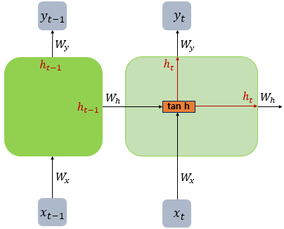
Where:

• x[t] is the input at time step t
• h[t] is the hidden state at time step t
• y[t] is the output at time step t

RNN cell (containing the weights and activation function)

The key equations governing the behavior of an RNN are:

1. Hidden state update: $h_t = \tanh(W_{hh}h_{t-1} + W_{xh}x_t + b_h)$

2. Output calculation: $y_t = W_{hy}h_t + b_y$

Where:

• $h_t$ is the hidden state at time t
• $x_t$ is the input at time t
• $y_t$ is the output at time t
• $W_{hh}$, $W_{xh}$, and $W_{hy}$ are weight matrices
• $b_h$ and $b_y$ are bias vectors
• $\tanh$ is the hyperbolic tangent activation function

Let’s break down these equations to understand what’s happening:

1. Hidden state update:

   • $W_{hh}h_{t-1}$: This term represents the influence of the previous hidden state. The weight matrix $W_{hh}$ determines how much of the previous state should be retained.
   • $W_{xh}x_t$: This term processes the current input. The weight matrix $W_{xh}$ determines how the current input should influence the hidden state.
   • $b_h$: This is a bias term, allowing the network to shift the activation function.
   • The $\tanh$ function squashes the sum of these terms to a range between -1 and 1, introducing non-linearity and helping to keep the values stable.

2. Output calculation:

   • $W_{hy}h_t$: This transforms the current hidden state into the output space.
   • $b_y$: Another bias term for the output.

The power of RNNs comes from their ability to maintain a “memory” of previous inputs through the hidden state, which is updated at each time step and influences future outputs.

Training RNNs: Backpropagation Through Time (BPTT)

Training RNNs involves a technique called Backpropagation Through Time (BPTT). This is an extension of the standard backpropagation algorithm used in feedforward networks, adapted to work with the temporal nature of RNNs.

The basic steps of BPTT are:

1. Forward pass through the entire sequence
2. Compute the loss
3. Backward pass through the entire sequence
4. Update the weights

The loss gradient with respect to the weights is accumulated over all time steps:

$\frac{\partial L}{\partial W} = \sum_{t=1}^T \frac{\partial L_t}{\partial W}$

Where $L$ is the total loss and $L_t$ is the loss at time step t.

BPTT can be thought of as “unrolling” the RNN through time and then applying standard backpropagation. Here’s a more detailed look:

1. In the forward pass, we compute the hidden states and outputs for each time step, storing the results.

2. We then compute a loss function that measures the difference between our predictions and the true values.

3. In the backward pass, we compute the gradient of the loss with respect to each parameter, working backwards from the last time step to the first. This is where the “through time” part comes in – we’re propagating the error back through the temporal structure of the network.

4. The gradients from each time step are summed to get the final gradient for each weight.

5. Finally, we update the weights using an optimization algorithm like gradient descent.

The key challenge in BPTT is handling long sequences, as the gradients can become very small (vanishing gradient problem) or very large (exploding gradient problem) when propagated over many time steps.

Challenges in Training RNNs

While powerful, RNNs face some challenges during training:

1. Vanishing Gradients: As the network processes long sequences, gradients can become extremely small, making it difficult for the network to learn long-term dependencies.

2. Exploding Gradients: Conversely, gradients can also become extremely large, causing instability during training.

3. Long-Term Dependencies: Standard RNNs often struggle to capture dependencies over long sequences.

To address these challenges, several variants of RNNs have been developed:

Long Short-Term Memory (LSTM) Networks

LSTMs introduce a more complex cell structure with gates to control the flow of information:

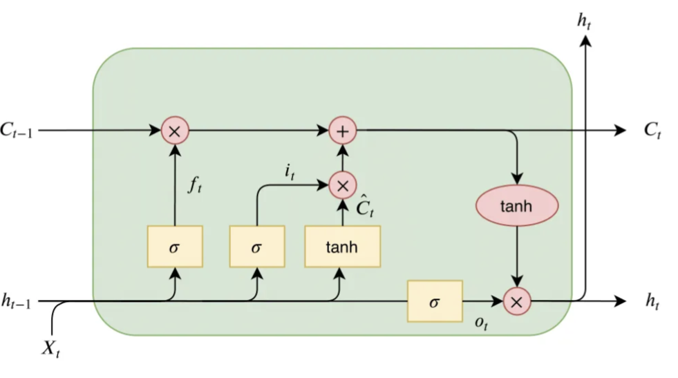
• Forget gate: $f_t = \sigma(W_f \cdot [h_{t-1}, x_t] + b_f)$
• Input gate: $i_t = \sigma(W_i \cdot [h_{t-1}, x_t] + b_i)$
• Output gate: $o_t = \sigma(W_o \cdot [h_{t-1}, x_t] + b_o)$
• Cell state update: $C_t = f_t * C_{t-1} + i_t * \tanh(W_C \cdot [h_{t-1}, x_t] + b_C)$
• Hidden state update: $h_t = o_t * \tanh(C_t)$

Where $\sigma$ is the sigmoid function and $*$ denotes element-wise multiplication.

LSTMs are designed to overcome the vanishing gradient problem. They do this by introducing a new state called the cell state $C_t$, which acts as a conveyor belt of information flowing through the network. The LSTM can add or remove information from the cell state, carefully regulated by structures called gates. Let’s break down each component:

1. Forget gate ($f_t$): This gate decides what information to throw away from the cell state. It looks at $h_{t-1}$ and $x_t$, and outputs a number between 0 and 1 for each number in the cell state $C_{t-1}$. A 1 represents “keep this” while a 0 represents “forget this.”

2. Input gate ($i_t$): This gate decides which new information we’re going to store in the cell state. It has two parts:

   • A sigmoid layer that decides which values we’ll update.
   • A tanh layer that creates a vector of new candidate values that could be added to the state.

3. Cell state update: We multiply the old state by $f_t$, forgetting the things we decided to forget earlier. Then we add $i_t * \tilde{C}_t$. This is the new candidate values, scaled by how much we decided to update each state value.

4. Output gate ($o_t$): This gate decides what we’re going to output. This output will be based on our cell state, but will be a filtered version.

5. Hidden state update: Finally, we update the hidden state, which is a filtered version of the cell state.

The beauty of this architecture is that the cell state provides a direct avenue for information to flow through the network without being substantially changed, which helps with learning long-term dependencies.

Gated Recurrent Units (GRUs)

GRUs simplify the LSTM architecture while maintaining many of its advantages:

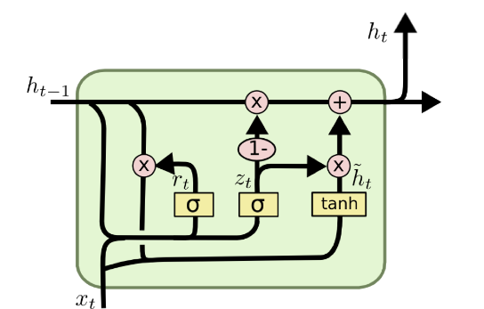
• Update gate: $z_t = \sigma(W_z \cdot [h_{t-1}, x_t])$
• Reset gate: $r_t = \sigma(W_r \cdot [h_{t-1}, x_t])$
• Candidate hidden state: $\tilde{h_t} = \tanh(W \cdot [r_t * h_{t-1}, x_t])$
• Hidden state update: $h_t = (1 - z_t) * h_{t-1} + z_t * \tilde{h}_t$

GRUs are a simpler variant of LSTMs, combining the forget and input gates into a single “update gate”. They also merge the cell state and hidden state.

1. Update gate ($z_t$): This gate decides how much of the past information (from previous time steps) needs to be passed along to the future. It can be thought of as the combination of the forget and input gates in an LSTM.

2. Reset gate ($r_t$): This gate is used to decide how much of the past information to forget.

3. Candidate hidden state ($\tilde{h}_t$): This is a new hidden state candidate, created using the reset gate to determine how much of the past state to incorporate.

4. Hidden state update: The final hidden state is a linear interpolation between the previous hidden state and the candidate hidden state, with the update gate determining the mix.

The main advantage of GRUs over LSTMs is that they’re computationally more efficient due to having fewer parameters. In practice, both GRUs and LSTMs tend to yield comparable results, with the best choice often depending on the specific dataset and task.